Large-Scale Load Stabilization
Results of experimental and numerical investigations of a permeable round parachute with the stripe-stabilizer, the so called "SAL" parachute - Stabilization of Aerodynamic Loads, are given [1].
Experimental investigations of a round parachute model with an additional stripe for stabilization have been carried out in the Grand Aerodynamic Wind Tunnel at the Institute of Mechanics of the Moscow State University. This parachute model was designed with 24-triangular gores manufactured of sections cut from woven parachute cloth of air- permeability parameter l about 800 l/m2s with a vent and sewed stripe for stabilization (so called stripe-stabilizer) on the suspension lines (in the same plane), on a short distance from a canopy edge.
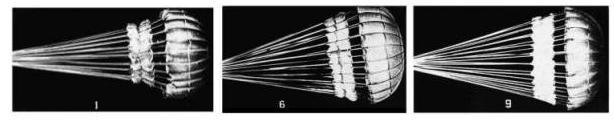
The model has the following parameters: a number of suspension lines - 24, the vent radius 26 cm, length distance between canopy edge and stripe-stabilizer 13 cm, stripe width 28 cm, length of lines 175 cm, the total length of reefing cord, passed through the middle of a stripe, D0= 426 cm. Nine various stages of reefing have been considered in the course of the tests: (cord of reefing was being shortened up to length D with a step of 30 cm). For each reefed parachute variant all loads were being measured at the confluence point at air flow velocities V= 10, 15, 20, 25, 30, 35 m/s. The parachute canopy attained different shapes from each other depending on the value of reefing (Fig.1).
|
|
In Fig.2 values of a drag coefficient are represented by different experimental symbols according to the upstream flow velocity via various parameters of reefing D = Dp/D0. Drag coefficient Cp = F/(rv2/2)S is related to a canopy surface area without stripe-stabilizer area, where F is the aerodynamic load, acting on the canopy, q = rv2/2 is aerodynamic pressure of the upstream flow, S is the total area of the main canopy. Values D corresponding to numbers of reefing variants: D = 0.366 corresponds to number 1; D = 0.47 - to number 2; , D = 0.93 - to number 9.
As given below some numerical investigations of the stripe-stabilizer reefing influence on the canopy shape, its aerodynamic drag and the tension of radial ribbons are considered.
The system of differential equations for the solution of this problem conformably to the considered parachute model was used [2]. This system describes the equilibrium of any radial ribbon element of a round parachute canopy:
 (1)
(1)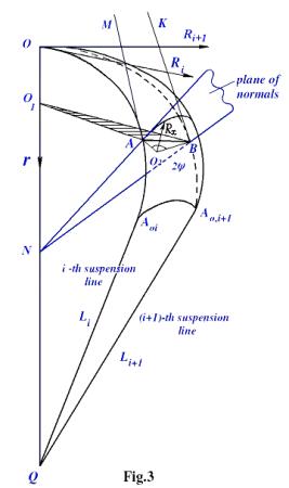
where T is a tension of the radial ribbon; S is a coordinate along the radial ribbon from the pole to the edge; q is the angle between tangent, plotted to meridional section, and the canopy axis; Rx is the radius curvature of the canopy element, stretched between the neighbouring radial ribbons based on the angle 2f. Rx is in the plane of normals, the angle between them is x. There is a complete system of differential equations (1) and (2) with unknown T, q, R, r and the following boundary conditions of the problem:
at the coordinate origin, i.e. on the canopy pole, tangent to meridional section is perpendicular to canopy axis. Therefore q(0) = p/2; R(0) = 0, r(0) = 0, but the value of tension T(0) on the pole is unknown. On the canopy edge the tangent coincides with suspension lines, i.e.
S = Sp/So , T = Tp/qS2, Rx = Rpx/So , r = rp/So , R = Rp/So , Dp= Dpp/q .
So is the radius of a round canopy in the plane of cutting out, index p means just parachute. Angles f, y, x and the radius curvature Rx are determined from the algebraic equations:
f = p/n, Rsin(f) = Rxsin(y), fS = yRx , sin(x) = sin(f)cos(q).
The formulated one-parameter boundary value problem has been solved by Newton's method [3]. Tension value T(0) is selected on the pole so that a given value of the line length would be obtained on the canopy edge. For a numerical integration of differential equations Runge-Kutta's method of the fourth order precision [4] has been used.
This problem was solved assuming Dp = const over the total canopy of parachute. The value of Dp for the considered parachute model with the known value of air-permeability was assigned by the constant value along the radial ribbon equal to 1.2.
from which one can see that D asymptotically tends to 1 (one), when L tends to infinity (that is the case when the diameter of stripe, tightened by the reefed cord, is equal to the diameter of the inlet). This relation was being put into boundary condition (3). Then the problem was being solved as if for an usual round parachute.
The values of the drag coefficient Cp have been obtained at all values of the reefing D as a result of the numerical solution of equations taking into account the above relation - the solid curve in Fig.2. One can see that scattering between numerical and experimental data of Cp is within by 3 - 8%.
Reefed canopy profiles obtained from the solution of the differential equations are shown in Fig.5 for parameters of the reefing 0.2 < D < 0.85 (with a step of the reefing 0.05). Having compared these profiles with photos of the corresponding canopies, one can notice their qualitative correspondence. For the quantitative comparison of experimental and numerical profiles the table of the ratio of S radial ribbon length divided by inlet radius R is shown below.
| reef.# | D | V, m/s | Snum/Rnum | Sexp/Rexp | % |
| 1 | 0.40 | 25 | 2.07 | 2.17 | 4.8 |
| 2 | 0.50 | 15 | 1.96 | 1.91 | 3.0 |
|
|
|
|
|
|
|
|
|
|
|
|
|
|
|
|
|
|
|
|
|
|
|
|
|
|
|
|
|
|
|
|
|
|
|
|
|
|
|
|
|
|
One can see from the right column
that the ratio of numerical S/R to experimental, does not exceed
5%. Satisfactory agreement of the experimental and numerical values of
Cp
and also the shape parameters of considered parachute indicates that one
may use the developed computer program.
Numerical distributions of radial
ribbon tension T are shown in Fig.6 within
0.2 < D < 0.8.
|
|
|
|
CONCLUSION
- first, to find out that the availability of the stripe-stabilizer (sewed fabric stripe on suspension lines) provides a good stable behaviour of the model in the flow;
- second, to determine the optimum value of reefing D = 0.648 for that average value of drag coefficient equal to 0.55;
- third, to reveal that drag coefficient Cp is practically invariable when value of reefing increases from D = 0.648; within 0.366 < D < 0.577 values of Cp are considerably smaller: 0.28 < D < 0.5.
REFERENCES
- M.V. Dzhalalova, A.F. Zubkov Numerical and Experimental Research of Permeable Parachute - SAL, Report #4400, MSU, Institute of Mechanics,1995, p.42.
- Kh.A. Rakhmatulin Theory of Axisymmetric Parachute, Transactions #35, Moscow State University, 1975.
- B.P. Demidovich, I.A. Maron Foundation of Computational Mathematics, Moscow, 1960.
- N.S. Bakhvalov Numerical Methods, Moscow, 1973.